  1
  2
  3
  4
  5
  6
  7
  8
  9
 10
 11
 12
 13
 14
 15
 16
 17
 18
 19
 20
 21
 22
 23
 24
 25
 26
 27
 28
 29
 30
 31
 32
 33
 34
 35
 36
 37
 38
 39
 40
 41
 42
 43
 44
 45
 46
 47
 48
 49
 50
 51
 52
 53
 54
 55
 56
 57
 58
 59
 60
 61
 62
 63
 64
 65
 66
 67
 68
 69
 70
 71
 72
 73
 74
 75
 76
 77
 78
 79
 80
 81
 82
 83
 84
 85
 86
 87
 88
 89
 90
 91
 92
 93
 94
 95
 96
 97
 98
 99
100
101
102
103
104
105
106
107
108
109
110
111
112
113
114
115
116
117
118
119
120
121
122
123
124
125
126
127
128
129
130
131
132
133
134
135
136
137
138
139
140
141
142
143
144
145
|
// Copyright https://mangoroom.cn
// License(MIT)
// Author:mango
// Histogram Equalization
// this is HistogramEqualization.cpp
#include <iostream>
#include<opencv2/opencv.hpp>
#include<array>
namespace imageprocess
{
// gray histogram
void GrayHistogram(const cv::Mat& gray_image, std::array<int, 256>& histogram);
// Histogram equalization
void HistogramEqualization(const std::array<int, 256>& histogram, std::array<int, 256>& out, int pixels_cout);
// histogram array to Mat
void Histogram2Mat(const std::array<int, 256>& histogram, cv::Mat& histogram_mat);
}//namespace imageproccess
int main()
{
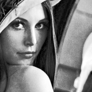
cv::Mat src_image = cv::imread("Fig0222(a)(face).tif", cv::IMREAD_GRAYSCALE);
if (src_image.empty())
{
return -1;
}
std::array<int, 256> histogram = { 0 };
std::array<int, 256> new_histogram = { 0 };
std::array<int, 256> dst_histogram = { 0 };
imageprocess::GrayHistogram(src_image, histogram);
cv::Mat histogram_mat;
cv::Mat cdf;
cv::Mat new_histogram_mat;
cv::Mat dst_image = src_image.clone();
imageprocess::HistogramEqualization(histogram, new_histogram, src_image.rows * src_image.cols);
imageprocess::Histogram2Mat(histogram, histogram_mat);
imageprocess::Histogram2Mat(new_histogram, cdf);
// adjust the origin image pixels
for (size_t i = 0; i < src_image.rows; i++)
{
for (size_t j = 0; j < src_image.cols; j++)
{
dst_image.at<uchar>(i, j) = new_histogram.at(src_image.at<uchar>(i, j));
}
}
imageprocess::GrayHistogram(dst_image, dst_histogram);
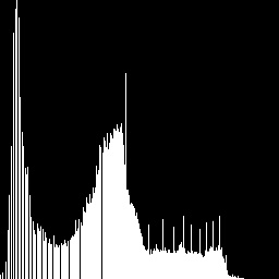
imageprocess::Histogram2Mat(dst_histogram, new_histogram_mat);
cv::imshow("src-image", src_image);
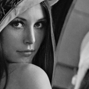
cv::imshow("dst-image", dst_image);
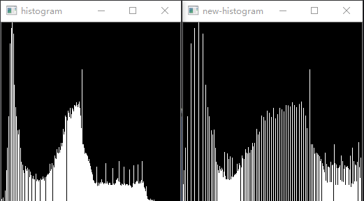
cv::imshow("histogram", histogram_mat);
cv::imshow("new-histogram", new_histogram_mat);
cv::imshow("cdf", cdf);
cv::imwrite("src-image.jpg", src_image);
cv::imwrite("dst-image.jpg", dst_image);
cv::imwrite("histogram.jpg", histogram_mat);
cv::imwrite("new-histogram.jpg", new_histogram_mat);
cv::imwrite("cdf.jpg", cdf);
cv::waitKey(0);
return 0;
}
void imageprocess::HistogramEqualization(const std::array<int, 256>& histogram, std::array<int, 256>& out, int pixels_cout)
{
// check the input parameter
assert(!histogram.empty() && !out.empty());
// calculate the new histogram (cdf)
out.at(0) = histogram.at(0);
for (size_t i = 1; i < 256; i++)
{
out.at(i) = out.at(i - 1) + histogram.at(i);
}
// create the look up table
for (size_t i = 0; i < 256; i++)
{
out.at(i) = static_cast<int>(255.0 * out.at(i) / pixels_cout);
}
}
void imageprocess::GrayHistogram(const cv::Mat& gray_image, std::array<int, 256>& histogram)
{
// check the input parameter : 检查输入参数
assert(gray_image.channels() == 1);
assert(histogram.size() == 256);
// step1: All elements of the histogram array are assigned a value of 0 : 将数组histogram所有的元素赋值为0
histogram = { 0 };
// step2: Do hf[f(x,y)]+1 for all pixels of the image: 对图像所有元素,做hf[f(x,y)]+1
for (size_t i = 0; i < gray_image.rows; i++)
{
for (size_t j = 0; j < gray_image.cols; j++)
{
int z = gray_image.at<uchar>(i, j);
histogram.at(z) += 1;
}
}
}
void imageprocess::Histogram2Mat(const std::array<int, 256>& histogram, cv::Mat& histogram_mat)
{
// Check the input parameter :检查输入参数
assert(histogram.size() == 256);
// step1: calculate the row of mat : 计算mat的row值
int row = 0;
for (size_t i = 0; i < histogram.size(); i++)
{
row = row > histogram.at(i) ? row : histogram.at(i);
}
// step2: initialize mat : 初始化mat
histogram_mat = cv::Mat::zeros(row, 256, CV_8UC1);
// step3: assign value for mat : 为mat赋值
for (size_t i = 0; i < 256; i++)
{
int gray_level = histogram.at(i);
if (gray_level > 0)
{
histogram_mat.col(i).rowRange(cv::Range(row - gray_level, row)) = 255;
}
}
// step4: resize the histogram mat : 缩放直方图
cv::resize(histogram_mat, histogram_mat, cv::Size(256, 256));
}
|
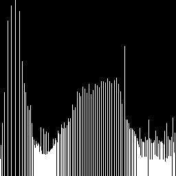
 (2) 形成图像直方图:扫描每个像素,增加相应的H成员,当像素p具有亮度$g_p$d时,做
$$H[g_p]=H[g_p]+1$$
(2) 形成图像直方图:扫描每个像素,增加相应的H成员,当像素p具有亮度$g_p$d时,做
$$H[g_p]=H[g_p]+1$$
 说明:以上便是求取直方图的运算,注意直方图无需归一化,此处直方图表示的是每个灰度级出现的次数而非概率。
(3)形成累积的直方图$H_c$:
$$H_c[0] = H_c[0]$$
$$H_c[p] = H_c[p-1] + H[p] \quad p = 1,2,…,G-1$$
说明:以上便是求取直方图的运算,注意直方图无需归一化,此处直方图表示的是每个灰度级出现的次数而非概率。
(3)形成累积的直方图$H_c$:
$$H_c[0] = H_c[0]$$
$$H_c[p] = H_c[p-1] + H[p] \quad p = 1,2,…,G-1$$
 说明:以上便是将直方图做离散的积分运算得到的累积直方图,即cdf(同样没归一化),此步为均衡化的关键步骤,由公式可知,将$H_c[p]$灰度级出现次数做调整得到一个新的$H_c[p]$。实际上此步骤已经得到了新的灰度值直方图,接下来的步骤是将新直方图应用到图像中。
(4)置$T[p] = round(\frac{G-1}{NM}H_c[p])$。这一步骤构造了一个是MN倍数的与单调增加的$H_c$中的值对应的查找表,有助于提高实现的效率。
说明:以上便是将直方图做离散的积分运算得到的累积直方图,即cdf(同样没归一化),此步为均衡化的关键步骤,由公式可知,将$H_c[p]$灰度级出现次数做调整得到一个新的$H_c[p]$。实际上此步骤已经得到了新的灰度值直方图,接下来的步骤是将新直方图应用到图像中。
(4)置$T[p] = round(\frac{G-1}{NM}H_c[p])$。这一步骤构造了一个是MN倍数的与单调增加的$H_c$中的值对应的查找表,有助于提高实现的效率。
 说明:此步的输入为一个灰度值$p$, 结果输出为一个新的灰度值。分两步来理解,首先$\frac{H_c[p]}{NM}$为归一化运算,为$p$的出现概率。然后$(G-1)\times\frac{H_c[p]}{NM}$,灰度级乘以概率得到新的灰度值。至此就完成了一个像素点灰度值的调整。